Warning

This documentation will no longer be mantained. The official FARGO3D repository is now https://github.com/FARGO3D/fargo3d, and the documentation is https://fargo3d.github.io/documentation/

Boundaries

Boundary conditions in FARGO3D can be selected only for the Y and Z directions, since in X the mesh is always considered periodic. It is because FARGO3D was mainly designed for azimuthal-periodic planetary disks, with a cost-effective orbital advection (aka FARGO) algorithm. Albeit that this limitation may seem strong in practice, there are lots of situations where you can assume your 3D problem to be periodic along a given direction. If you can not do that, unfortunately there is no way to avoid this limitation with the present version of the code.

The boundary conditions (BCs) are handled by the script boundparser.py. We have developed a metalanguage to handle them. Although this may seem quite a futile investment, it soon appeared to be much needed as we were developing the code. We had initially left the treatment of BCs on the CPU, even for GPU builds. We thought that the filling of the ghost zones by the CPU would have negligible impact on the overall speed of the code. This, however, turned out to be untrue: the CPU-GPU communication overhead, and the slowness of CPU calculations lowered the code performance significantly. We therefore decided to deal with BCs in the exact same way as with other time consuming routines, which can be translated automatically to CUDA, so as to run on the GPU. This implied some syntax constraints on the associated C code, which would have made the development of a variety of boundary conditions on the four edges of the mesh a time consuming and error prone process (yes, four, because they are specified only for Y and Z). For this reason, we have chosen to write a script that produces the C code for a given set of boundary conditions, with all the syntactic comments needed to subsequently translate it to CUDA.

How are boundary conditions applied?

The boundary conditions are applied just after the initialization of a specific SETUP (before the first output), and subsequently, twice per time step. Boundary conditions are applied to all primitive variables, and to the electromotive forces (EMFs). All boundary conditions are managed by the routine FillGhosts(), inside src/algogas.c. Below, we depict schematically how cells of the active mesh are mapped to the ghost zones.

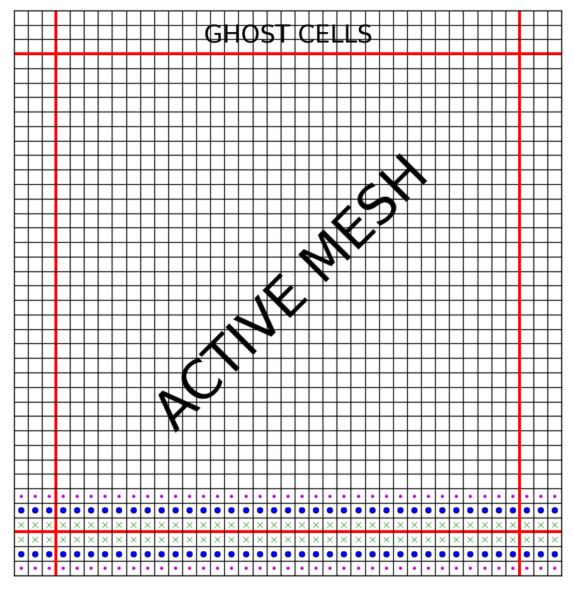
Schematic view of how the boundaries are applied. We note that the buffer (or ghost) zones are three cells wide.

The last (third) ghost cell is filled with the first active one, the second ghost cell is filled with the second active one, and finally, the first ghost cell is filled with the third active cell.

Note

Note that we do not consider the mesh periodicity along a given direction as a proper boundary condition, in the sense that no ad hoc prescription has to be used to fill the corresponding ghost zones. Rather, a mesh periodic along a given dimension has no boundary in this dimension, and this property is assigned to the mesh in the parameter file (and not in the boundary files of the setup that we present in detail below) by the use of the Boolean parameters PeriodicY and PeriodicZ, which default to NO. In the boundary files that we present hereafter, you will therefore see BC labels such as SYMMETRIC, OUTFLOW, etc., but never PERIODIC.

Note

In the figure above we have three rows of ghost cells. The number of rows depends on the problem, and on how frequently communications are performed within a time step. There is a trade-off between the number of rows (large buffers slow down the calculations and the communications) and the number of communications. The number of ghosts is defined in src/define.h around line 40 et sq.

boundparser.py

In order to work with boundaries, we have developed a script called boundparser.py, that reads a general boundary text file and converts it into a C file, properly commented to be subsequently converted into a CUDA file. boundparser.py works with four files, called:

• setup.bound

• boundaries.txt

• centering.txt

• boundary_template.c

(note: these last three files can be in your setup directory, or by default, the script takes those of the std/ directory, as prescribed by the VPATH variable.)

boundparser.py reads the information inside the setup.bound file, and compares it with the information in boundaries.txt and centering.txt. Finally, it builds a set of C files that apply the boundary conditions (called [y/z][min/max]_boundary.c) with a proper format, given by boundary_template.c. We will not give a detailed description on how boundparser.py works, but it is not difficult to understand the script if you are interested in its details.

The key to developing boundary conditions is to understand the structure of setup.bound and boundaries.txt file. Both files are in the same format, described below.

Boundaries files format

boundaries.txt, centering.txt and setup.bound files have the same format. All are case-insensitive, and have two levels of information: the main level and an inner level. Also, comment lines are allowed. The general structure of the format is:

# Some header
#--------

LEVEL1_a:
        Level2_a: Some_data1_a   #A comment
        Level2_b: Some_data1_b
        Level2_c: Some_data1_c
        Level2_d: Some_data1_d

# A comment line

LEVEL1_b:
        Level2_a: Some_data2_a
        Level2_b: Some_data2_b
        Level2_c: Some_data2_c
        Level2_d: Some_data2_d


etc...

centering.txt

Special care must to be taken to the centering of data. Not all data are defined at the same location in FARGO3D. In order to write automatically boundary conditions in a given direction (Y/Z), it is necessary to know which fields are centered or staggered in this direction. This information is taken by boundparser.py from centering.txt. This file uses the same format described above, and uses a particular set of instructions. The allowed values are:

• LEVEL1 –> The name of a Field Structure inside the code (eg: Density, Vx, Bz, etc…).

• Level2 –> the word “Staggering”

• data –> C,x,y,z or a combination of xyz (eg: xy, yz, xyz)

C is short of “centered”, meaning that the field is a cube-centered quantity. The meaning of x is staggered in x, that is to say the corresponding quantity is defined at an interface in x between two zones, rather than in the middle of two subsequent interfaces. By default, the field value is assumed centered along each direction that does not appear explicitly in the centering definition.

Let us have a look at some lines of centering.txt:

Density:

Staggering: C

Bz:

Staggering: z

Emfz:

Staggering: xy

The first two lines specify that the density is a cube centered quantity. The following two lines specify that the magnetic field in the z-direction is centered in x and y, but staggered in z (ie defined at the center of an interface in z). Finally, the last two lines indicate that the EMF in z is centered in z, but staggered in x and y. It is, therefore, a quantity defined at half height of the lower vertical edge in x and y of a cell.

All primitive variables and the EMF fields are defined by default in std/centering.txt. If you create a new primitive field in the code, you should specify its correct centering in std/centering.txt if you want to create boundary conditions for this field.

boundary_template.c

This file is taken as a template for building automatic boundary condition C files . You should never have to deal with it. Also, it contains all the information for subsequent building of the CUDA files. If you need special boundary conditions, you could try modifying this file first. As long as you do not alter the lines beginning with “%”, you can modify this template. This kind of modification should be made by an advanced user.

boundaries.txt

This file is the core file for the boundary condition. The main idea is to provide a way to the user to define a boundary prescription in as user-friendly a manner as possible. Let us begin with a simple example. Assume that we want to define a boundary condition that we call SYMMETRIC, which simply consists in copying the data of the active cell into the ghost zone. We represent schematically what is intended on this diagram:

|           |           |
|           |           |
      ^           ^
      |           |
    ghost       active
    zone         zone

The active zone contains a value, that we call, arbitrarily, active

|           |   active  |
|           |           |
      ^           ^
      |           |
    ghost       active
    zone         zone

We want to set the value of the ghost zone to the same value, that is we want:

|  active   |   active  |
|           |           |
      ^           ^
      |           |
    ghost       active
    zone         zone

Therefore we represent this boundary condition with the following, rather intuitive line of code:

|  active  |  active  |

Assuming for the moment that this boundary condition applies to centered variables, we would finally write the following piece of code in boundaries.txt to define our SYMMETRIC boundary condition:

SYMMETRIC:
      Centered:    |  active  |  active  |

The right “cell” always represent the active cell, and the left “cell” the corresponding ghost cell. The string active could be actually any string:

SYMMETRIC:
      Centered:    |  value  |  value  |

If we wish to have an anti-symmetric boundary condition (that is to say that we set the ghost value to the negative of its active counterpart):

|  -active  |   active  |

Should we want to set the ghost value to twice the active zone’s value:

|  2.0*foo  |   foo  |

Or if we wish to set it to some predefined value (say that you have a supersonic flow of uniform, predefined density 0.12 g/cm^3 entering the mesh, and you work in cgs):

|  0.12  |   whatever  |

in which case the value whatever is never used. Naturally, it is much better to use a parameter (say, RHO0, that you define in your parameter file):

|  'RHO0'  |   whatever  |

We shall come back to the use of the quotes later on in this section.

This, in a nutshell, is how we define boundary conditions in the code.

Now, assume that we want to have an anti-symmetric boundary condition on the velocity perpendicular to the boundary. The situation is a bit different than the one described above, because this field is staggered along the dimension perpendicular to the mesh. That is, we have:

|        |||        |
|        |||        |
          ^       value
          |
         edge of
       active mesh

As shown on this diagram, the value is defined at the interface, and not at the center as previously. The triple vertical line delineates the edge of the active mesh. What we intend is the following:

  |        |||        |
  |        |||        |
-value      ^       value
            |
           edge of
         active mesh

but this leaves yet unspecified the value at the edge of the active mesh, which should be set here to zero (it has to be its own negative):

  |        |||        |
  |        |||        |
-value      0       value

Eventually, we have to specify one extra value with respect to the centered case. Our boundary condition is therefore coded as:

ANTISYMMETRIC:
      Staggered:    |  -value  |  0  |   value  |

If the | (pipe) symbol could be thought of as representing the zones interface for the centered case, it is no longer the case in the staggered case. In any case, we will always have two “cells” in the BC code for a centered quantity, and three “cells” in the BC code for a staggered quantity, regardless of the number of rows in the ghosts. The matching between an active cell and its corresponding ghost zone is as shown on the figure at the beginning of this section.

We sum up this information: the file boundaries.txt contains a two level description that obeys the general following rule:

• LEVEL1 –> the name of the boundary. It is an arbitrary name, defined by you.

• Level2 –> the word “Centered” or “Staggered”, followed by some data.

• data –> |some_text_1|some_text_2| or |some_text_1|some_text2|some_text3|

The rules in the ghost zone are as follows:

1. Any string used in the active zone that matches some part of the ghost zone string will be replaced by the active cell value.

2. Any string inside '' will be textually parsed and converted to upper-case. They are useful to match the parameters of the parameter files, which are upper-case C variables.

3. Any string that does not match rule 1 nor rule 2, will be textually parsed and converted to lower case.

Additionally, there is a set of indices helpers, for working with boundaries:

*jgh/kgh: The index of the y/z ghost cells.
*jact/kact: The index of the y/z active cells.

These helpers prove very useful to perform complex extrapolations at the boundaries. You can see examples in the file std/boundaries.txt.

Examples:

Zero-gradient boundary:

Suppose we want to define a zero gradient boundary. That means we want to copy all the active zone in the ghost zone for both centered and staggered meshes.

The syntax is as follows. It groups together the definitions that we have worked out above, for centered and staggered fields:

SYMMETRIC:
           Centered:     |active|active|
           Staggered:    |active|active|active|

where the right active value will be copied without any modification to the ghost zone. Note that this boundary definition is direction and side independent, ie it can apply to ymin, ymax, zmin and zmax.

Keplerian extrapolation example

We define here a more complex boundary condition:

KEPLERIAN2DDENS:
          Centered:            |surfdens*pow(Ymed(jact)/Ymed(jgh),'SIGMASLOPE')|surfdens|

This line is equivalent to:

KEPLERIAN2DDENS:
          Centered:            |active*pow(ymed(jact)/ymed(jgh),'sigmaslope')|active|

as per the rules listed above.

What kind of action does this instruction correspond to ? It sets the value of the ghost zone to:

\(\mbox{ghost value}=\Sigma_\textrm{active}\left(\frac{R_\textrm{act}}{R_\textrm{ghost}}\right)^\alpha\)

since Ymed stands for the radius of the center of zone, in a cylindrical setup.

The reader familiar with protoplanetary disk’s jargon and notation will easily recognize the radial extrapolation of the surface density of the disk in the ghost zone, with a power law of exponent \(-\alpha\) (\(\alpha\) is dubbed SIGMASLOPE in the parameters of FARGO3D), hence the string chosen to represent the value of the active cell (surfdens), although at this stage nothing specifies yet to which variable this boundary condition should be applied. This is the role of the file SETUP .bound.

SETUP.bound

This file must be located in the sub-directory of a given setup, and must have same prefix as the setup to which it refers. For instance, in setup/fargo/, the file that specifies the boundaries is called fargo.bound.

The files that we described in the previous paragraphs are used to specify what transformation rule is used for an arbitrary field (in boundaries.txt) depending on its centering, while the centering of all fields is specified by std/centering.txt.

The SETUP .bound file now specifies the transformation rule to use for each physical variable. It obeys the following general syntax:

• LEVEL1 –> The name of the field.

• Level2 –> The side of the boundary (ymin,ymax,zmin,zmax), and some data.

• data –> Boundary label (the label defined in boundaries.txt)

We show hereafter a few examples:

2D XY reflecting problem

We want to have a 2D isothermal fluid with periodic “boundary conditions” in X (as required in FARGO3D) and reflecting boundary conditions in Y.

We have three primitive variables to which we must apply BCs. Those will only apply in Y (not in X because of the periodicity, nor in Z because we have a 2D X-Y setup).

The setup.bound file should therefore look similar to:

Density:
        Ymin:   SYMMETRIC
        Ymax:   SYMMETRIC

Vx:
        Ymin:   SYMMETRIC
        Ymax:   SYMMETRIC

Vy:
        Ymin:   ANTISYMMETRIC
        Ymax:   ANTISYMMETRIC

where Vy is ANTISYMMETRIC in Y because we have reflection in the y-direction.

At build time, the script boundparser.py goes through this file. The first three lines instruct it to generate C code to implement a boundary condition for the density field in ymin and ymax. It goes to the definition of SYMMETRIC found in std/boundaries.txt. Two definitions are available: one for centered fields, the other one for staggered fields. In std/centering.txt it finds that the density is centered (in y) and therefore generates the C code corresponding to the centered case. The same thing occurs for Vx: it finds that this field is centered in Y. Finally, the last three lines instruct it to generate C code for an ANTISYMMETRIC boundary condition of Vy in Y. It finds in std/centering.txt that this field is staggered in Y, and generates the C code corresponding to the definition:

| -value | 0 | value |

The C functions thus produced contain all the comments required to further conversion to CUDA, should the user request a GPU built.

2D YZ reflecting problem

Now, a more complex example, with all directions (yet in 2D):

Density:
        Ymin: SYMMETRIC
        Ymax: SYMMETRIC
        Zmin: SYMMETRIC
        Zmax: SYMMETRIC

Vx:
        Ymin:   SYMMETRIC
        Ymax:   SYMMETRIC
        Zmin:   SYMMETRIC
        Zmax:   SYMMETRIC

Vy:
        Ymin:   ANTISYMMETRIC
        Ymax:   ANTISYMMETRIC
        Zmin:   SYMMETRIC
        Zmax:   SYMMETRIC

Vz:
        Ymin:   SYMMETRIC
        Ymax:   SYMMETRIC
        Zmin:   ANTISYMMETRIC
        Zmax:   ANTISYMMETRIC

Note

Note how the staggering is implicit in Vy/Vz boundaries.

An extensive list of examples can be found in the setups/ directory.

Common errors

This section will be developed later from users’ feedback.

The boundparser.py script is at the present time a bit taciturn, and may silently ignore errors which might be a bit difficult to spot afterward. Among them:

• Incorrect names or misprints.

• An incorrect centering.

Defining boundaries by hand

Sometimes more flexibility is needed when creating boundaries. You can always define the boundaries by hand by disabling the parser that creates the boundaries.

In order to create the boundary sources manually, you can proceed as follows:

1. Create the ymin_bound.c, ymax_bound.c, etc… files manually:

   > cd scripts
   > python boundparser.py ../std/centering.txt ../std/boundaries.txt ../setups/yoursetup/yoursetup.bound
   

The previous instruction produces the boundary files (in scripts/) called ymin_bound.c, ymax_bound.c, etc…, needed to build the executable.

2. Copy the newly created boundary source files into your setup directory.

3. Comment the following lines in the makefile:

   %_bound.o: ymin_bound.c ${GLOBAL}
      @${COMPILER} $*_bound.c -c ${INCLUDE} ${OPTIONS} ${FARGO_OPT}
   
   ymin_bound.c: ${BOUNDARIES} ${GLOBAL}
      @echo PARSING BOUNDARIES...
      @-python ${SCRIPTSDIR}/boundparser.py $^
   
   ymax_bound.c zmin_bound.c zmax_bound.c: ymin_bound.c
   

4. Modify the boundary source files manually.

5. build the executable (make) and check if the boundaries were indeed compiled from your setup directory, e.g:

   ...
   CC ../setups/fargo/ymin_bound.c ==> ymin_bound.o
   CC ../setups/fargo/ymax_bound.c ==> ymax_bound.o
   CC ../setups/fargo/zmin_bound.c ==> zmin_bound.o
   CC ../setups/fargo/zmax_bound.c ==> zmax_bound.o
   ...
   

Note

Since the version 2.0, the .opt option FARGO_OPT += -DHARDBOUNDARIES has been added to make the steps 3,4 and 5 automatically.