Warning

This documentation will no longer be mantained. The official FARGO3D repository is now https://github.com/FARGO3D/fargo3d, and the documentation is https://fargo3d.github.io/documentation/

Default SETUPS

FARGO3D was developed with simulations of protoplanetary disks in mind but it is a sufficiently general code to tackle a lot of different problems. This property makes that its ancestor, the public code FARGO, is simply a particular case of the wide range of possible setups that can be designed.

This section contains a brief summary of the setups that come with the public version of FARGO3D. We develop in more detail the setup called fargo.

We emphasize that a setup must not be confused with a set of parameters, those being provided in a so-called parameter files (with extension .par, by convention). A setup corresponds to a given physical problem and geometry: in a setup we specify the grid geometry, the equation of state to be used, whether we use the MHD module. etc. In the parameter file we give specific values for a given setup, such as the mesh size, parameters specific of the initial conditions, etc. A given setup can be run with many different parameter files without recompiling. Usually one file only is required to run FARGO3D once it has been build for a given setup. This file is the parameter file. There is an exception with some setups, like the fargo setup, which in addition require a file in which the planetary system initial configuration is specified. The planet files (which by convention have the extension .cfg) have the exact same syntax as in the former FARGO code, so planetary systems designed for a prior FARGO calculation can be used straight away. There are located in the sub-directory planets of the main directory. Their name and path must be passed to the code through the string parameter PLANETCONFIG.

fargo

This setup is a legacy setup. The public FARGO code, ancestor of FARGO3D, amounts to this particular setup of FARGO3D. This is the default setup, and the initial conditions are taken from one of the EU comparison setups. The setup is strictly comparable to the template.par parameter file of the FARGO code.

We explain some special characteristics of the fargo setup:

Make options

This setup uses the following physical options, which are selected in the file setups/fargo/fargo.opt:

• X

• Y

• CYLINDRICAL

• ISOTHERMAL

• VISCOSITY

• POTENTIAL

• STOCKHOLM

It also activates the following flag:

• LEGACY

which requests the output of two files dumped by the former FARGO code: dims.dat and used_rad.dat, which can be needed by certain reduction scripts.

As can be seen also in the .opt file, it has the monitoring of the:

• MASS

• MOM_X

• TORQ

We shall come back to the monitoring of quantities later on in this manual

Parameters

The following parameters are essentially the same as those of the FARGO code. You can also browse the online help of that code to get the detail of each of them.

• Setup: This keyword specifies the name of the setup that should be used to build the code in order to run this parameter file. If it is left unspecified, this parameter file can be run using a build of FARGO3D with otvortex, mri, etc., with potentially surprising error message and outcomes.

• AspectRatio: (real). Sets the disk aspect ratio (\(h_0 = H/R_0\)) at \(r=R_0\), where \(R_0\) is a characteristic length, defined in src/fondam.h. It is a natural choice to use \(R_0=1\) in a scale free setup. Physically, this parameter is related to the sound speed through:

  \[\displaystyle{\frac{H}{r} = \frac{c_s}{\Omega_k r}}\]

  This parameter is a way to initialize a desired sound speed on the disk.

• Sigma0: (real) Sets the numerical value of the surface density at \(r=R0\).

• SigmaSlope: (real) Sets the exponent of the density profile, assumed to be a power law of radius:

\[\displaystyle{\Sigma(r) = \text{Sigma0}\left(\frac{r}{R_0}\right)^{\text{-SigmaSlope}}}\]

• FlaringIndex (real) Sets the flaring of the disk. If it is null, the aspect ratio of the disk is constant (ie, the disk height scales linearly with r). The dependence of the the aspect ratio with the flaring index is:

\[\displaystyle{h(r) = \frac{H}{r} = h_0\left(\frac{r}{R_0}\right)^{\text{FlaringIndex}}=\text{AspectRatio} \left(\frac{r}{R_0}\right)^{\text{FlaringIndex}}}\]

• PlanetConfig: (string) The name the planetary file to be used. The path is relative to the location at which you launch the code.

• ThicknessSmoothing: (real) Potential smoothing length for all the planets. The use of this parameter is mutually exclusive with the use of *RocheSmoothing*. The smoothing length \(s\) of the potential is “\(\text{ThicknessSmoothing} \times H\)”:

\[ \begin{align}\begin{aligned}\displaystyle{s = \text{AspectRatio} \times \left(\frac{r}{R_0}\right)^{\text{FlaringIndex}}\times r \times \text{ThicknessSmoothing}}\\\text{The potential of a planet of mass $m_p$ has the form: } \displaystyle{\phi = -\frac{Gm_p}{\sqrt{r^2+s^2}}, \text{where $r$ is here the distance to the planet.}}\end{aligned}\end{align} \]

• RocheSmoothing: (real) Potential smoothing length for all the planets. The use of this parameter is mutually exclusive with the use of ThicknessSmoothing. The smoothing length of the potential over the mesh is “\(\text{RocheSmoothing} \times R_h\)”, there \(R_h\) is the Hill radius of the current planet:

\[\displaystyle{s = \text{RocheSmoothing}\times r\times \left(\frac{m_p}{3M_{star}}\right)^{1/3}}\]

• Eccentricity: (real) The initial eccentricity of all the planets.

• ExcludeHill: (boolean) When this parameter is set to YES, a cut-off is introduced when the force is computed. The cut-off is calculated with the formula:

  \[ \begin{align}\begin{aligned}h_c = 0 \;\;\;\text{ if } r/r_{Hill} < 0.5\\h_c = 1 \;\;\;\text{ if } r/r_{Hill} > 1.0\\h_c = \sin^2\left[\pi \left(r/r_h - 1/2 \right)\right] \;\;\;\text{ otherwise }\end{aligned}\end{align} \]

  and the force is cut off prior to the torque calculation (see src/compute_force.c):

  \[F_{\text{cut off}} = F \times h_c\]

Note

This parameter needs the make option called HILLCUT to be activated in the .opt file (it is because this cut is somehow expensive on the GPU). This is achieved by adding this line to the setups/fargo/fargo.opt file: FARGO_OPT += -DHILLCUT

IndirectTerm: (boolean) Selects if the calculation of the potential indirect term that arises from the primary acceleration due to the planets’ (and possibly the disk’s) gravity is performed. In the fargo setup, the reference frame is by default centered on the central star (see also Removing the default central star). For this reason, this parameter should normally be set to yes. If the preprocessor macro GASINDIRECTTERM is undefined, the indirect term only arises from the planet’s acceleration imparted to the primary. If, on the contrary, this macro is defined, the acceleration imparted to the primary by the disk is also taken into account. Defining this macro can be done in the .opt file using the line: FARGO_OPT += -DGASINDIRECTTERM.

Frame: (string) Sets the reference frame behavior: F (Fixed), C (Corotating) and G (Guiding center) (it is case insensitive). When it is set to F, the frame rotates at a constant angular speed, specified by OmegaFrame. When it is set to Corotating, the frame corotates with planet number 0. If this planet migrates or has an eccentric orbit, the frame angular speed is not constant in time. When it is set to Guiding-Center, the frame corotates with the guiding-center of planet 0. The frame angular speed, therefore, varies with time if the planet 0 migrates, and it does so in a smoother manner than in the Corotating case.

OmegaFrame: (real) It is the angular velocity of the reference frame. It has sense only if the parameter Frame is equal to F (Fixed).

boundaries

Because this problem is 2D in XY, only boundary conditions in Y are applied. The boundary conditions are an extrapolation of the Keplerian profile for the azimuthal velocity, the density is also extrapolated using its initial power law profile, and an antisymmetric boundary condition on the radial velocity is applied.

If STOCKHOLM is activated (in the .opt file), the wave-killing recipe of De Val-Borro (2006) is used to damp disturbances near the mesh boundaries in radius (or colatitude for more general setups such as p3diso). The width of the margin over which a wave killing boundary condition is applied near a boundary is defined by the parameters DampingZone for the radial boundaries and KillingBCColatitude for the boundaries in colatitude. The former represents the ratio of the orbital periods between the edge of the wave-killing zone and the corresponding edge of the mesh. The default value of 1.15 implies that the wave-killing zones have a width approximately equal to 10% of the radius of the mesh edge (\(1.15^{2/3}\approx 1.10\)). KillingBCColatitude represents the fraction of the angle between the mesh limit and the midplane over which the damping prescription is applied. It defaults to 0.2. You can use a value smaller than one for DampingZone to suppress the wave-killing boundary condition at radial boundaries, and you can use a negative value for KillingBCColatitude to suppress this prescription in the boundary in colatitude.

In Cylindrical setups, no damping is applied in the Z-boundary if the setup is periodic along that direction (such as in unstratified MRI), and a 10% margin is applied otherwise. This is hardcoded in src/stockholm.c.

Note

It is not recommended to use a wave-killing boundary condition in colatitude when a gap-opening planet is present in the disk: replenishing the gas at high altitude tends to prevent the opening of the gap. At the very least, if a wave-killing boundary condition is used in this case, it should not be applied on the density (the corresponding line should be commented out in src/stockholm.c).

Note

the default value of 1.15 for DampingZone is smaller than the recommended value of 1.5 found by Benitez-Llambay et al. (2016, ApJ, 826, 13). Using this value would require much larger radial ranges for the meshes of the public setups provided in the distribution. As a consequence, a minute amount of wave reflection may be noticed with these setups even when the wave-killing prescription is activated.

Orszag-Tang Vortex

This setup corresponds to the well known 2D periodic MHD setup of Orszag and Tang, widely used to assess the properties of MHD solvers. We briefly go through the make options of the .opt file and through the parameter file.

Make options

Here are the options activated in the .opt file:

• X

• Y

• Z

• MHD

• STRICTSYM

• ADIABATIC

• CARTESIAN

• STANDARD

• VANLEER

The first four lines are self-explanatory.

Note

Even though the Orszag-Tang setup is a 2D setup, every time the MHD is included, all three dimensions should be defined. This is why we define here X, Y, and Z.

The flag STRICTSYM on the fifth line is meant to enforce a strict central symmetry of the scheme. Usually, after some time (the amount of time depends on the resolution) the central vortex begins to drift in some direction, breaking the initial central symmetry of the setup. It can be desirable to check whether this break of symmetry arises as a consequence of amplification of noise, or because the scheme contains a bug that renders it non-symmetric. We have found that, at least on the CPU, asymmetries in the scheme arise from additions of more than two terms, which are non-commutative. As the MHD solver implies, at several places, arithmetic averages of four variables, we need to group them by two in order to enforce symmetry. If the initial conditions are strictly symmetric, the fields will then remain symmetric forever. The interested reader may “grep” STRICTSYM in the sources. This trick does not work on the GPUs on which we have tested it, however.

The other make flags have already been discussed in the fargo setup.

Parameters

The parameter file is short and each of its variables is self-explanatory.

Suggested run

You may activate run time visualization to see the vortex evolve (you must have installed matplotlib for that):

$ make SETUP=otvortex GPU=0 PARALLEL=1 view
$ mpirun -np 4 ./fargo3d setups/otvortex/otvortex.par

Sod shock tube 1D

This very simple setup is self-explanatory. You may obtain information about it by issuing at the command line:

make describe SETUP=sod1d

If you build it with run-time visualization, a graph of a field is displayed in a matplotlib window. This field is selected by the variable Field of the parameter file.

MRI

The setup mri (lower case) corresponds to an MHD turbulent unstratified disk on a cylindrical mesh, periodic in Z, much similar to the setup of Papaloizou and Nelson 2003, MNRAS 339, 983. The data provided in this public release have the same coverage and resolution as the data by Baruteau et al. 2011 A&A, 533, 84. We present hereafter in some detail the make options and the parameter file, and we provide a hands-on tutorial on reducing data from this setup.

Make options

The file setups/mri/mri.opt shows that the following options are defined at build time:

• FLOAT

• X, Y, Z, MHD

• ISOTHERMAL

• CYLINDRICAL

• POTENTIAL

• VANLEER

The FLOAT option runs everything that is related to the gas in single precision (should we have planets, their data would remain in double precision). This speeds up by a factor ~2x the simulation, both on CPUs and GPUs.

The other flags have already been explained in the previous setups. We note that here, counter to what was set in otvortex, we do not request the STANDARD flag for orbital advection. Therefore, by default, the scheme will use the fast orbital advection (aka FARGO) described for hydrodynamics by Masset (2000), A&ASS, 141, 165, and for the EMFs by Stone & Gardiner, 2010, ApJS, 189, 142.

Parameter file

This parameter file, as said earlier, corresponds to the “disks” contemplated in Baruteau et al (2011), with a radial range from 1 to 8 and from -0.3 to 0.3 in z, half a disk in azimuth, and an “aspect ratio” of 0.1 (the word aspect ratio is misleading here; it merely imply that \(c_s=0.1v_k\) everywhere in the disk). Besides, the mesh is rotating so as to have its corotation at r=3. The initial \(\beta\) of the gas is 50, and the initial magnetic field is toroidal (see setups/mri/condinit.c). Some shot noise is introduced on the vertical and radial components of the velocity, with an amplitude of NOISE percent of the local sound speed (therefore here 5%).

Some Ohmic resistivity is introduced (see Induction equation). As there is a file called nimhd_ohmic_diffusion_coeff.c in the setup directory, it supersedes the same file in the src directory. We see that this file implements a linear ramp of resistivity near each radial boundary, of radial width 1/7th of the radial extent, hence here of radial width 1.

Hands on test

We hereafter run the setup for 300 orbits at the disk’s inner edge, and examine some statistical properties of the turbulence that arises.

To start with, we forget any prior build option of the code:

make mrproper

We then build the mri setup. Owing to the computational cost, it is a good idea to run it on one or several GPUs. In what follows, we take the example of a run on one GPU. The run takes about 10 hours to complete on one Tesla C2050. You can degrade the resolution to speed things up during your first try.

It is a good idea, also, to tune the CUDA block size prior to running the setup (you may skip this part if you wish). Execution will be 10-20% faster.:

make blocks setup=mri

Note that everything is lower case in the line above. It will take a few minutes to complete. Upon completion, issue:

make clean
make SETUP=mri GPU=1

and the code is built using the block size information previously determined, or using a default block size (architecture independent) if you skipped the action above.

We now start the run:

./fargo3d -t in/mri.par

The t option above activates a timer that will give you an idea of the time it takes to complete a run.

You can see that there are several files in the output directory (presumably outputs/mri if you have not changed this value of the variable OUTPUTDIR in the parameter file), called respectively:

• reynolds_1d_Y_raw.dat

• maxwell_1d_Y_raw.dat

• mass_1d_Y_raw.dat

that grow in size progressively, every time a carriage return is issued after a line of “dots” [1]. This kind of file is presented in detail in the section Monitoring later on in this manual. For the time being, it suffices to know that these are raw, binary 2D files, to which a new row is added every DT (fine grain monitoring). This row contains radial information (as indicated by the _Y_ component of the file name: Y is the radius in cylindrical coordinates). Let us try and display one of these files (with Python). We start ipython directly from the output directory:

$ ipython --pylab
...
In[1]: n = 10  #assume you have reached 10 outputs. Your mileage may vary.
In[2]: ny=320 #Radial resolution. Adapt to your needs if you altered the par file
In[3]: m=(fromfile("reynolds_1d_Y_raw.dat",dtype='f4'))[:n*10*ny].reshape(n*10,ny)
In[4]: imshow(m,aspect='auto',origin='lower')
In[5]: colorbar()

Note

A few comments about these instructions. In the third line we read the binary file “reynolds_1d_Y_raw.dat” and specify explicitly with the dtype keyword that we are reading single precision floating point data (fromfile otherwise expects to read double precision data). The trailing [:n*10*ny] truncates the long 1D array of floating point values thus read up to the row value number n*10 (10 because this is the value of NINTERM). This 1D array is finally reshaped into a 2D array, plotted on the following line

You should see a figure such as:

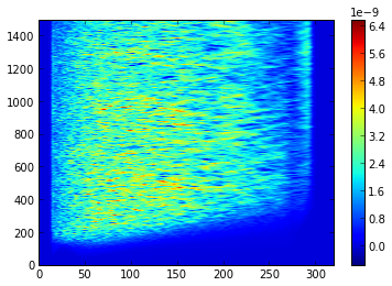
Figure obtained with the above Python instructions (here with n=150, ie upon run completion)

On this plot, the x-direction represents the radius, whereas in the y-direction we pile up the radial profiles that have been dumped every DT. Therefore the y-direction represents the time. If we remember that the file name has radix reynolds, we are obviously looking at some quantity related to the Reynold’s stress tensor, and we see how turbulence develops in the inner regions and progresses toward larger radii as time goes on. But what is exactly the quantity that we plot ?

It is:

\[\displaystyle{R(r)\Delta r = \int_\phi rd\phi\int_z dz\rho v_r(v_\phi-\overline{v_\phi}) \Delta r}\]

That is to say, it is the sum in \(z\) and in \(\phi\) of the quantity:

\[\displaystyle{\rho v_r(v_\phi-\overline{v_\phi})\times\mbox{ cell volume} }\]

This quantity is evaluated in src/mon_reynolds.c and it is subsequently passed to the systematic machinery of Monitoring.

In the same vein, we can plot the quantities found respectively in maxwell_1d_Y_raw.dat and in mass_1d_Y_raw.dat. There are the vertical and azimuthal sum on all cells of the following quantities:

\[\displaystyle{\frac{B_rB_\phi}{\mu_0}\times \mbox{ cell volume}}\]

and

\[\displaystyle{\rho\times \mbox{ cell volume}}\]

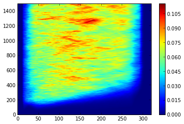
We see that the value of \(\alpha\) can therefore be obtained as follows:

r=(arange(ny)+.5)/ny*7+1
cs2 = 0.01/r
cs2array = cs2.repeat(10*n).reshape(ny,10*n).transpose()
reyn=(fromfile("reynolds_1d_Y_raw.dat",dtype='f4'))[:n*10*ny].reshape(n*10,ny)
maxw=(fromfile("maxwell_1d_Y_raw.dat",dtype='f4'))[:n*10*ny].reshape(n*10,ny)
mass=(fromfile("mass_1d_Y_raw.dat",dtype='f4'))[:n*10*ny].reshape(n*10,ny)
alpha_maxwell = -maxw / (mass * cs2array)
alpha_reynolds = reyn / (mass* cs2array)
alpha = alpha_maxwell + alpha_reynolds
imshow (alpha, aspect='auto', origin='lower'); colorbar ()

which gives the following picture:

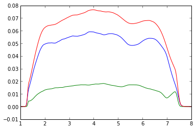
We plot the different time averaged values of \(\alpha\) once the turbulence has reached a saturated state:

plot(r,alpha_maxwell[500:,:].mean(axis=0))
plot(r,alpha_reynolds[500:,:].mean(axis=0))
plot(r,alpha[500:,:].mean(axis=0))

which gives the following plot:

We finally plot the radially averaged value of \(\alpha\) between r=2 and r=6 (corresponding to bins 46 to 228 in Y) as a function of time:

plot(arange(1500)*1.256,alpha[:,46:228].mean(axis=1))

which gives the following plot:

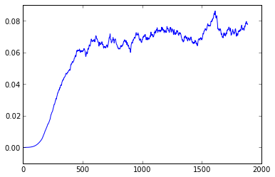
We see that we obtain a relatively substantial value for \(\alpha\) in this fiducial run (much larger than the one obtained with same parameters in the run with NIRVANA in Baruteau et al. (2011), at Fig. 6). One reason for that is the use of orbital advection, another one is the systematic use of the van Leer slopes in the upwind evaluation of all quantities involved in the MHD algorithm. Comparison with other code of the Orszag-Tang vortex at different resolutions corroborates this statement.

See also

Monitoring

[1]

Each dot stands for an elementary HD or MHD time step. The number of dots on a line (which has length DT) is given by the CFL condition.